Electrical Circuits
📚 Syllabus Alignment & Reading
- Scheduled Course Week: Week 4 — Lecture 08
- Reading: Irwin & Nelms (12th Ed.), Ch. 5: Sec. 5.3 (Thévenin's and Norton's Theorems)
- Module Learning Objective: Convert a source between its two equivalent forms, and reduce any linear network, at a chosen pair of terminals, to a single voltage source in series with a resistance — or, equivalently, to a single current source in parallel with the same resistance.
- Short period today. This is Part 1, and it reaches Norton — which costs two slides rather than a lecture, because once source transformation is in hand the Norton form is one step from the Thévenin one. Maximum power transfer is Part 2, on Tue Sep 22 (Lecture 09).
- EE 314 · Topic: Source Transformation, Thévenin and Norton
- ECE, UAB · Fall 2026
Hiding a Network Behind Two Terminals
- A load connected at a pair of terminals experiences exactly two things: the voltage across them and the current through them. It has no way to find out what produced them.
- So here is the question worth asking: can everything behind those terminals be replaced by something simpler that produces the same voltage and current, for every load? For a linear network the answer is yes — and two elements are enough.
- Irwin puts the scale of that plainly: "we could represent the entire U.S. power grid at a pair of terminals with one of the equivalent circuits."
🔧 Two tools, same idea
Source transformation works locally — swap one source-and-resistor pair for the other form, repeatedly, and watch the circuit collapse. Thévenin's theorem works globally — find two numbers and the whole network is done at once.
Source Transformation
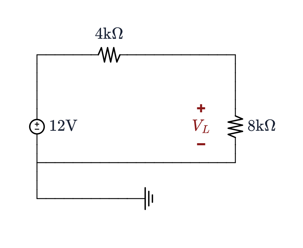
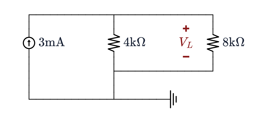
The two are interchangeable at their terminals whenever $\;\mathbf{v_S = R\,i_S}\;$ — here $12 = (4\text{k})(3\text{ mA})$ — and provided $R$ really sits in series with the voltage source and in parallel with the current one. A resistor anywhere else is not part of the pair and does not come along. The load then sees $8$ V and $1$ mA either way, so no measurement made outside can tell the two apart.
Inside, they are not the same circuit at all. The $4\ \text{k}\Omega$ carries $1$ mA on the left and $2$ mA on the right, dissipating $4$ mW against $16$ mW, and the source supplies $12$ mW against $24$ mW. Equivalence is a statement about the terminals and about nothing else — never use it to reason about internal power.
Worked Example 1: Collapse It From the Left
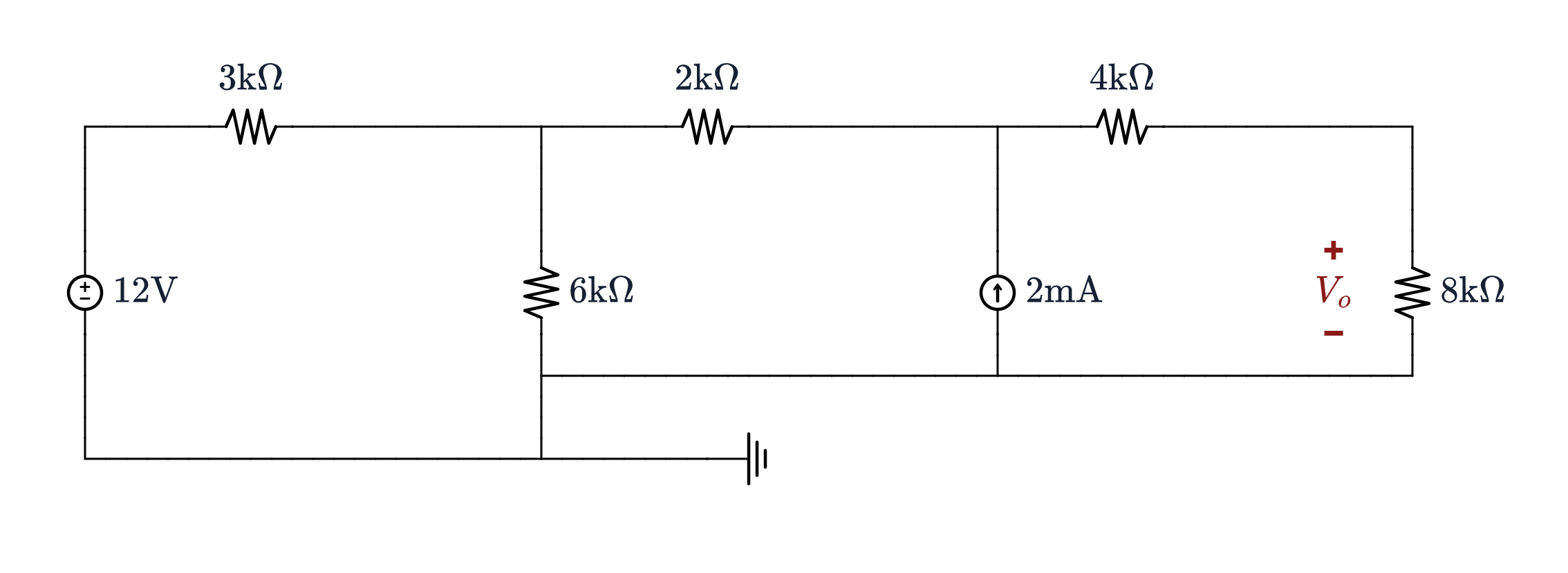
Find $V_o$, the voltage across the $8\ \text{k}\Omega$.
- Nodal analysis would give three equations in three unknowns. Nothing wrong with that — but there is a cheaper route here.
- Every source in this circuit already sits with a resistor in the right place. So transform the leftmost one, combine whatever becomes parallel or series, and repeat. The circuit gets shorter each time, and $V_o$ never changes, because every step is an equivalence at the terminals of everything to its right.
Step 1: The 12 V Source Becomes 4 mA
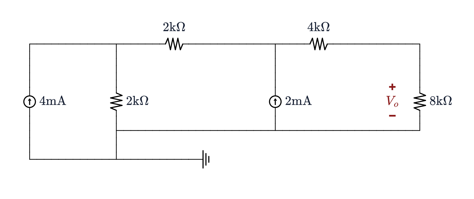
Transform: $12$ V behind $3\ \text{k}\Omega$ becomes $i_S = v_S/R = 12/3\text{k} = 4$ mA across $3\ \text{k}\Omega$.
Then combine: that $3\ \text{k}\Omega$ is now in parallel with the $6\ \text{k}\Omega$ that was already there, and $$3\text{k}\,\|\,6\text{k} = \frac{(3\text{k})(6\text{k})}{9\text{k}} = 2\ \text{k}\Omega$$
This is the pattern for the whole chain: transform, then combine. The transform on its own buys nothing — it is the combining afterwards that shortens the circuit.
Steps 2 and 3: Back, Then Forward Again
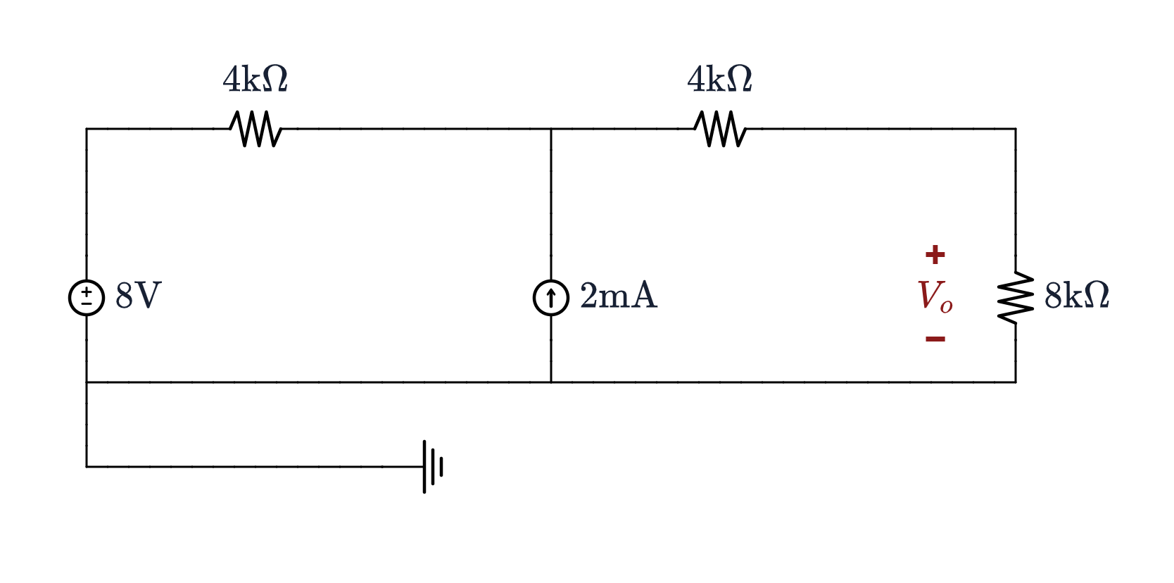
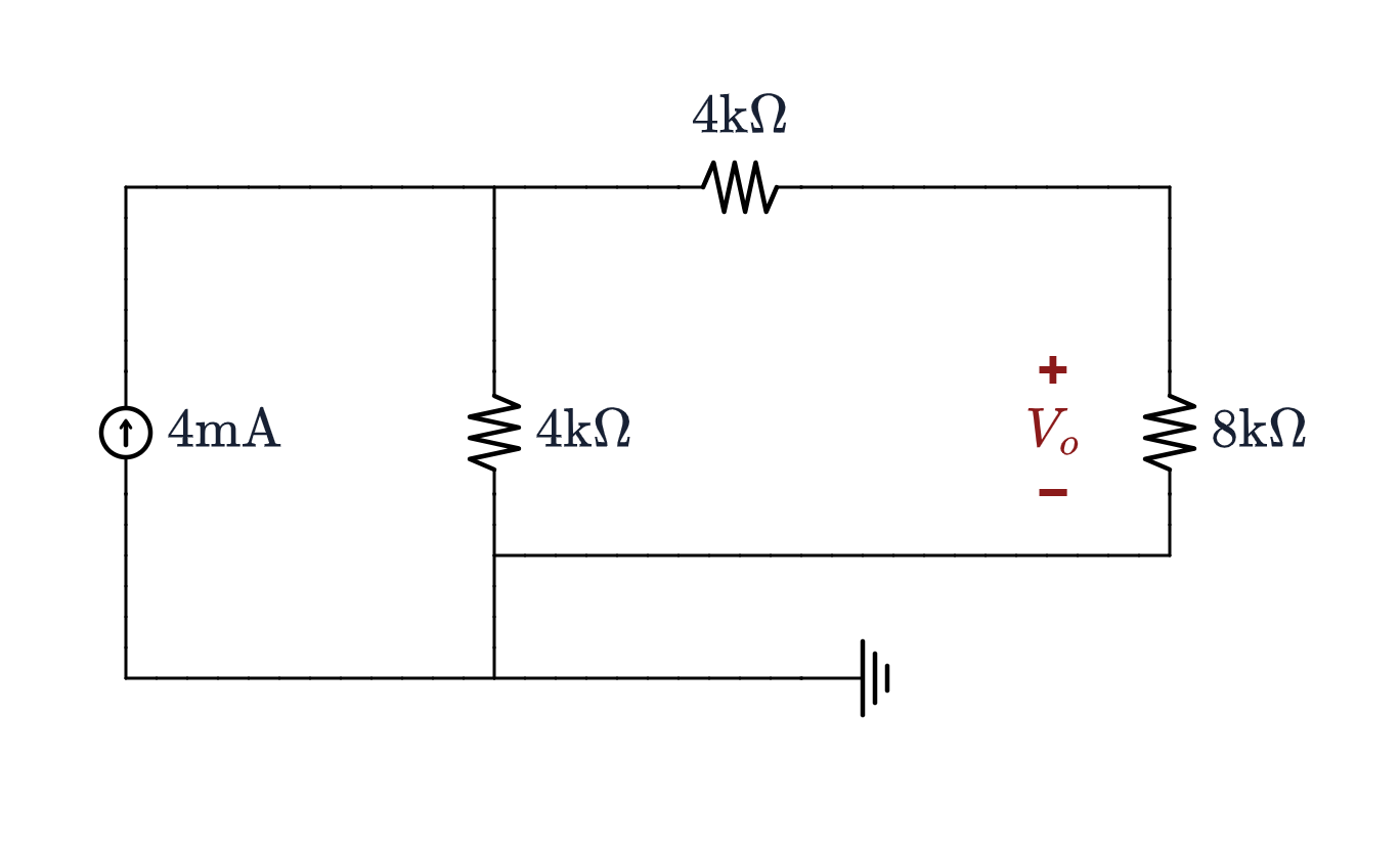
- Going back to a voltage source is not a step backwards. It was what let the two $2\ \text{k}\Omega$ merge into one, which a current source in that position could never have done.
- Then forward again, and the pay-off: two sources become one. Parallel current sources add, so $2 + 2 = 4$ mA. Seven elements are now three.
Finish, and Check
- What is left is a current source, a shunt and a divider: $$\begin{aligned} v &= (4\ \text{mA})\big(4\text{k}\,\|\,(4\text{k}+8\text{k})\big) = (4\ \text{mA})(3\ \text{k}\Omega) = 12\ \text{V} \\ V_o &= 12\left(\frac{8\text{k}}{4\text{k}+8\text{k}}\right) = \mathbf{8\ \text{V}} \end{aligned}$$
- Check against the original, by nodal analysis on the three-node circuit we started with: $$2V_1 - V_2 = 8, \qquad -2V_1 + 3V_2 - V_3 = 8, \qquad -2V_2 + 3V_3 = 0$$ which solves to $V_3 = 8$ V. ✓
- All four circuits in the chain give $V_o = 8$ V, because each was an exact equivalent of the last at the terminals of the $8\ \text{k}\Omega$. Open any of the four live pages and probe it.
Thévenin's Theorem
Any linear two-terminal network can be replaced, at those terminals, by a single voltage source $V_{Th}$ in series with a single resistance $R_{Th}$.
- "Linear" is the hypothesis, and it is the one Tuesday was about. Without it there is no theorem.
- "At those terminals" is the limitation. The equivalent reproduces the voltage and current at $a$–$b$ and makes no claim whatever about what happens inside — least of all about internal power.
- It is exact. Not a small-signal approximation, not valid only for large loads: the equivalent gives the right answer for every load, including a short and an open.
- So a network of any size collapses to two numbers. The rest of this lecture is how to find them.
The Two Numbers
| Number | How you get it |
|---|---|
| $V_{Th}$ | Remove the load and find the open-circuit voltage $V_{oc}$ across the terminals, by any method you like — divider, nodal, mesh, superposition. |
| $R_{Th}$ | (a) Only independent sources: set them all to zero — voltage
sources shorted, current sources opened — and combine the resistors that
remain. This is today's case. (b) Only dependent sources: apply a test source at the terminals and take the ratio of terminal voltage to terminal current. (c) Both: $R_{Th} = V_{oc}/I_{sc}$. |
- Case (a) is every circuit today, and slide 17 checks one by route (c). Case (b), and (c) with dependent sources in the network, are Tuesday's — Assignment 2 uses them.
Problem-Solving Strategy: Thévenin
- Remove the load and find the voltage across the open terminals, $V_{oc}$.
- Find $R_{Th}$ looking into those same open terminals, with the load still removed and the independent sources zeroed.
- Reconnect the load to $V_{oc}$ in series with $R_{Th}$, and solve. With a resistive load this is one voltage divider.
- Choose the break carefully. Anything can be the "load" — it is whatever you want to stop re-analysing. Break at the element you are asked about, or at the one whose value keeps changing.
- Steps 1 and 2 look at the same circuit with the load off. Draw it once, then do both.
Step 1: The Open-Circuit Voltage
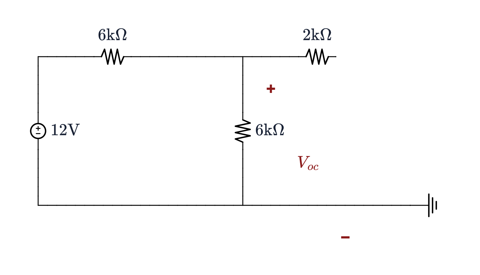
With $a$–$b$ open there is nowhere for current in the $2\ \text{k}\Omega$ to go, so it carries zero current — and therefore drops zero volts. Terminal $a$ sits at exactly the voltage across the $6\ \text{k}\Omega$ shunt:
$$V_{oc} = 12\left(\frac{6\text{k}}{6\text{k}+6\text{k}}\right) = \mathbf{6\ \text{V}}$$
The $2\ \text{k}\Omega$ has not been ignored. It is carrying no current, which is a different statement — and it will matter very much in the next step.
Step 2: The Thévenin Resistance
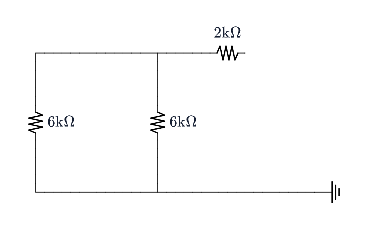
Shorting the $12$ V source ties the left end of the series $6\ \text{k}\Omega$ to the reference — so that resistor becomes a second shunt, sitting beside the original $6\ \text{k}\Omega$:
$$R_{Th} = (6\text{k}\parallel 6\text{k}) + 2\text{k} = 3\text{k} + 2\text{k} = \mathbf{5\ \text{k}\Omega}$$
Look into $a$–$b$ from the right: the two $6\ \text{k}\Omega$ are in parallel (both tie to the reference at the bottom, and their tops join), and the $2\ \text{k}\Omega$ sits in series between that combination and terminal $a$.
And now the $2\ \text{k}\Omega$ counts, because it lies in the path from $a$ to $b$. A resistor can carry no current in Step 1 and still dominate Step 2.
Step 3: Reconnect the Load
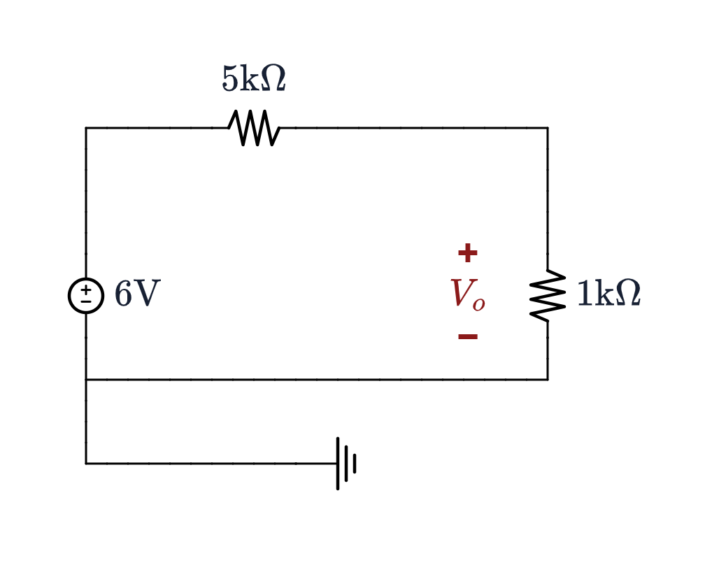
$V_{oc} = 6$ V in series with $R_{Th} = 5\ \text{k}\Omega$, with the $1\ \text{k}\Omega$ put back. One divider:
$$V_o = 6\left(\frac{1\text{k}}{1\text{k}+5\text{k}}\right) = \mathbf{1\ \text{V}}$$
Check against the original. Solving the four-element circuit from slide 11 directly — $12$ V, $6\text{k}$, $6\text{k}$, $2\text{k}$, $1\text{k}$ — also gives $V_o = 1$ V, with $1$ mA in the load. ✓
That agreement is also the check on $R_{Th}$: get the $5\ \text{k}\Omega$ wrong and the two answers part company immediately.
Norton's Theorem
Any linear two-terminal network can equally be replaced, at those terminals, by a single current source $I_N$ in parallel with a single resistance $R_N$.
The two equivalents are one source transformation apart — slide 3, run in the other direction: $$I_N = \frac{V_{Th}}{R_{Th}}, \qquad R_N = R_{Th}$$
Each number is a measurement at $a$–$b$: $V_{Th}$ is the open-circuit voltage $V_{oc}$, and $I_N$ is the short-circuit current $I_{sc}$ — short the terminals of the Norton form and all of $I_N$ flows through the short. Hence $R_{Th} = V_{oc}/I_{sc}$.
Norton for Worked Example 2
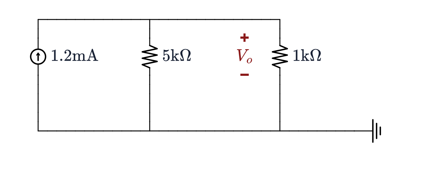
You have already built it. Worked Example 2 gave $V_{Th} = 6$ V and $R_{Th} = 5\ \text{k}\Omega$, so $$I_N = \frac{V_{Th}}{R_{Th}} = \frac{6}{5\text{k}} = 1.2\ \text{mA}, \qquad R_N = R_{Th} = 5\ \text{k}\Omega$$
So Norton is never a fresh derivation when you already have Thévenin, or the other way round. And the load agrees, for the third time: $V_o = (1.2\ \text{mA})(5\text{k}\,\|\,1\text{k}) = 1$ V, with $1$ mA in the $1\ \text{k}\Omega$. ✓
Norton Directly: the Short-Circuit Current
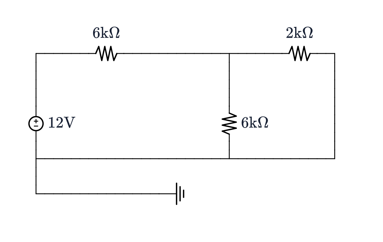
$I_N$ can also be found with no reference to Thévenin at all: short $a$–$b$, and measure the current through the short.
The short puts the $2\ \text{k}\Omega$ straight across the reference, so the middle node now sees $6\text{k}\,\|\,2\text{k} = 1.5\ \text{k}\Omega$: $$I_{src} = \frac{12}{6\text{k} + 1.5\text{k}} = 1.6\ \text{mA}$$ $$v_m = (1.6\ \text{mA})(1.5\text{k}) = 2.4\ \text{V}$$ $$I_{sc} = \frac{2.4}{2\text{k}} = \mathbf{1.2\ \text{mA}} = I_N\ \checkmark$$
That also hands you $R_{Th}$ a second way, for nothing: $$R_{Th} = \frac{V_{oc}}{I_{sc}} = \frac{6}{1.2\ \text{mA}} = 5\ \text{k}\Omega$$ the same $5\ \text{k}\Omega$, found without combining a single resistor. This is case (c) from slide 9 — and it is the route you will have to take once dependent sources are in the network.
Why Bother, and What Comes Next
For one load, Thévenin is no faster than nodal analysis. For a load that keeps changing, it is the only sane way to work:
| $R_L$ | $V_o = 6\,R_L/(R_L + 5\text{k})$ | Work needed |
|---|---|---|
| $1\ \text{k}\Omega$ | $1$ V | One divider each, once the equivalent exists. Without it, a full re-solve of the whole network per value. |
| $5\ \text{k}\Omega$ | $3$ V | |
| $10\ \text{k}\Omega$ | $4$ V |
💡 Part 2, Tuesday 22 September — from the next slide
Maximum power transfer. Given the equivalent, which $R_L$ draws the most power from it? The table above is already hinting at the answer — $V_o$ keeps climbing as $R_L$ grows, but the current keeps falling, so the product must peak somewhere in between.
Then the two harder routes to $R_{Th}$, cases (b) and (c) from slide 9, on networks containing dependent sources — which is what Assignment 2 will need.
Part 2 — Tuesday 22 September
Part 1 reduced any linear network, seen from two terminals, to one source and one resistor. Two questions were left open, and Assignment 2 — issued today — needs both answers.
💡 Where Part 1 stopped
- Which load? The sweep on the previous slide had $V_o$ climbing the whole way as $R_L$ grew, while the current fell. So the power must peak somewhere in between — where, and how much?
- Which $R_{Th}$? Every network so far had independent sources only, so $R_{Th}$ came from zeroing them and combining resistors. That route closes the moment a dependent source is in the network. Two others stay open.
Maximum Power Transfer: The Question
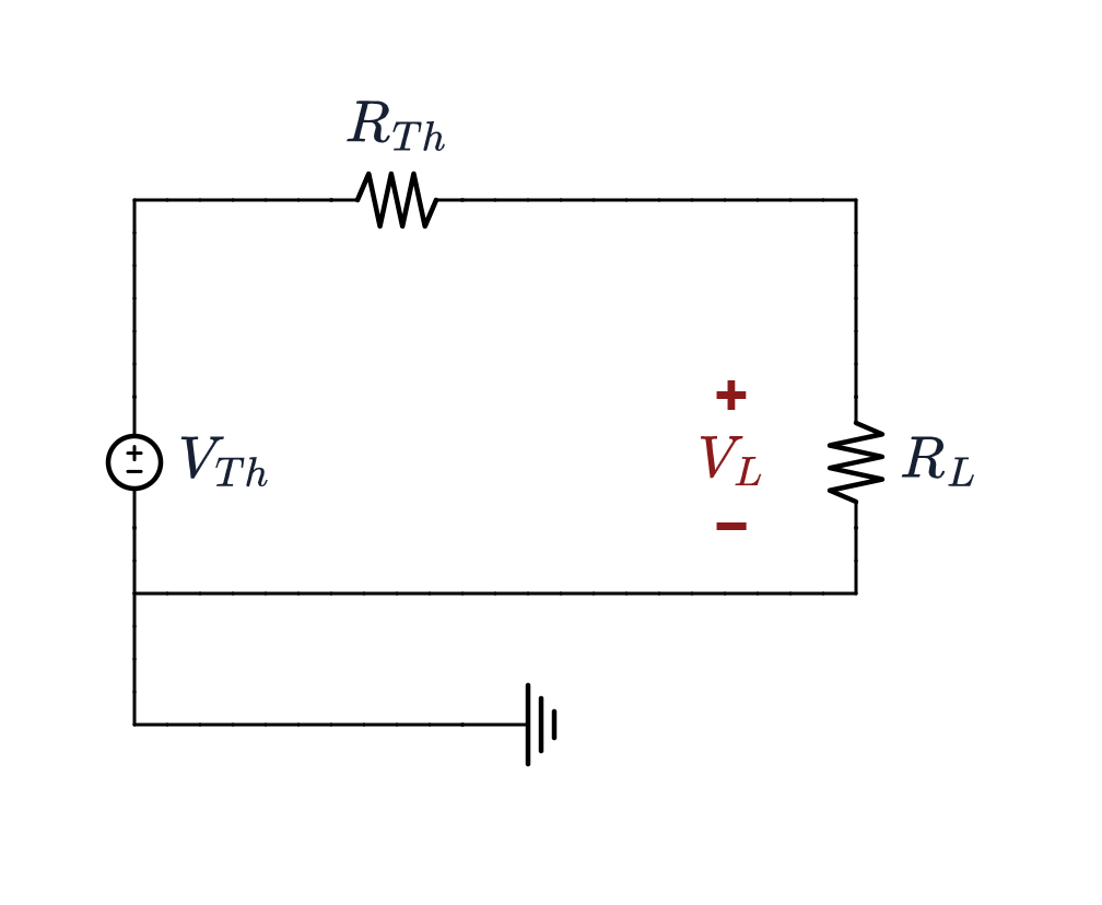
The source is fixed: $V_{Th}$ and $R_{Th}$ describe a network you cannot change. The load is yours to choose. One loop, so the current is a divider away:
$$i = \frac{V_{Th}}{R_{Th} + R_L} \qquad P_L = i^2 R_L = \frac{V_{Th}^{\,2}\,R_L}{(R_{Th} + R_L)^2}$$
- $R_L \to 0$: maximum current, but no voltage across the load. $P_L \to 0$.
- $R_L \to \infty$: the full $V_{Th}$ across the load, but no current. $P_L \to 0$ again.
- Zero at both ends and positive in between, so there is a maximum somewhere. Finding it is one derivative.
One Derivative, Step by Step
$P_L = V_{Th}^{\,2}\,R_L/(R_{Th}+R_L)^2$, and only $R_L$ moves. The peak is wherever the slope of that curve is zero, so differentiate with respect to $R_L$.
Step 1 — the tool, and the parts. $P_L$ is a fraction, so use the quotient rule; $V_{Th}^{\,2}$ is constant and comes along for the ride. $$\left(\frac{u}{v}\right)' = \frac{u'v - u v'}{v^2} \qquad \begin{aligned} u &= R_L &&\longrightarrow& u' &= 1 \\ v &= (R_{Th}+R_L)^2 &&\longrightarrow& v' &= 2(R_{Th}+R_L) \end{aligned}$$
Step 2 — put them into the rule. $$\frac{dP_L}{dR_L} = V_{Th}^{\,2}\,\frac{\overbrace{1}^{u'}\cdot(R_{Th}+R_L)^2 - \overbrace{R_L}^{u}\cdot\overbrace{2(R_{Th}+R_L)}^{v'}}{(R_{Th}+R_L)^4}$$
Step 3 — tidy up. Both terms on top carry a factor $(R_{Th}+R_L)$, so cancel one against the bottom: $$= V_{Th}^{\,2}\,\frac{(R_{Th}+R_L) - 2R_L}{(R_{Th}+R_L)^3} = V_{Th}^{\,2}\,\frac{R_{Th} - R_L}{(R_{Th}+R_L)^3}$$
The bottom is always positive, so the sign is the sign of $R_{Th}-R_L$ — climbing below the match, zero at it, falling above. A maximum, not a minimum: $\;\boxed{\;R_L = R_{Th}\;}\;$ and then $\;\boxed{\;P_{max} = V_{Th}^{\,2}/4R_{Th}\;}$
What the Curve Looks Like
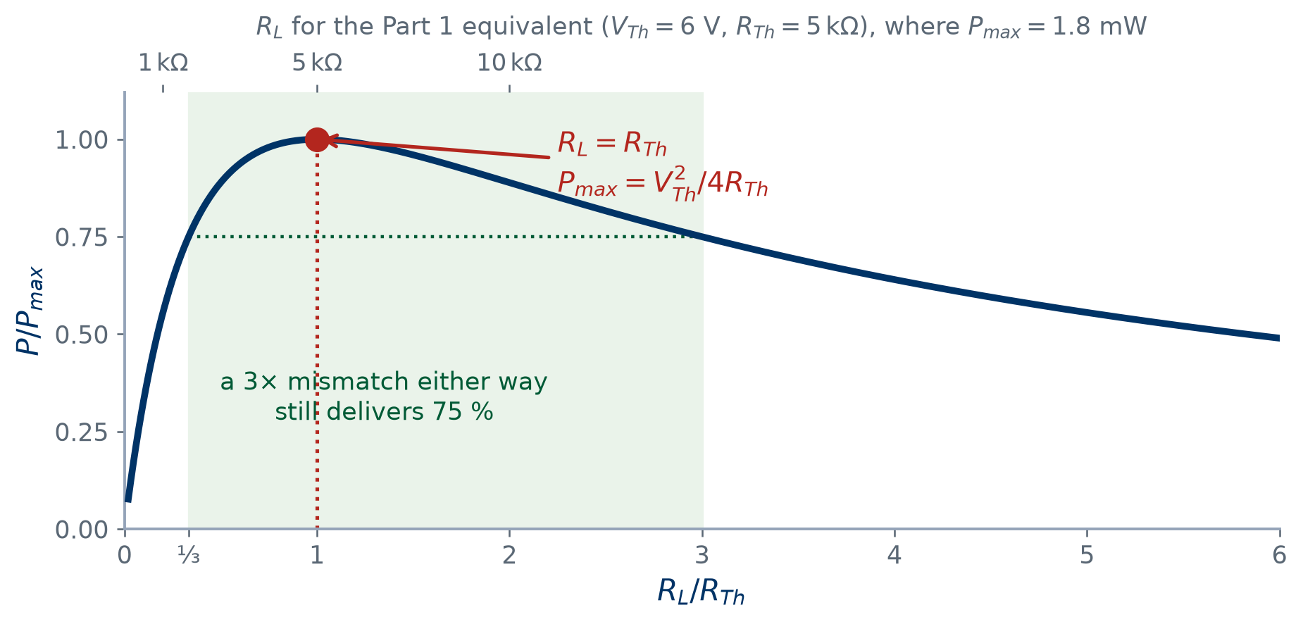
- The peak is broad: a load off by a factor of three, either way, still collects 75 % of the maximum. Matching is worth doing approximately and rarely worth doing precisely.
- Not symmetric, though — too small a load loses power fast, too large loses it slowly.
Worked Example 3: Back to Part 1's Equivalent
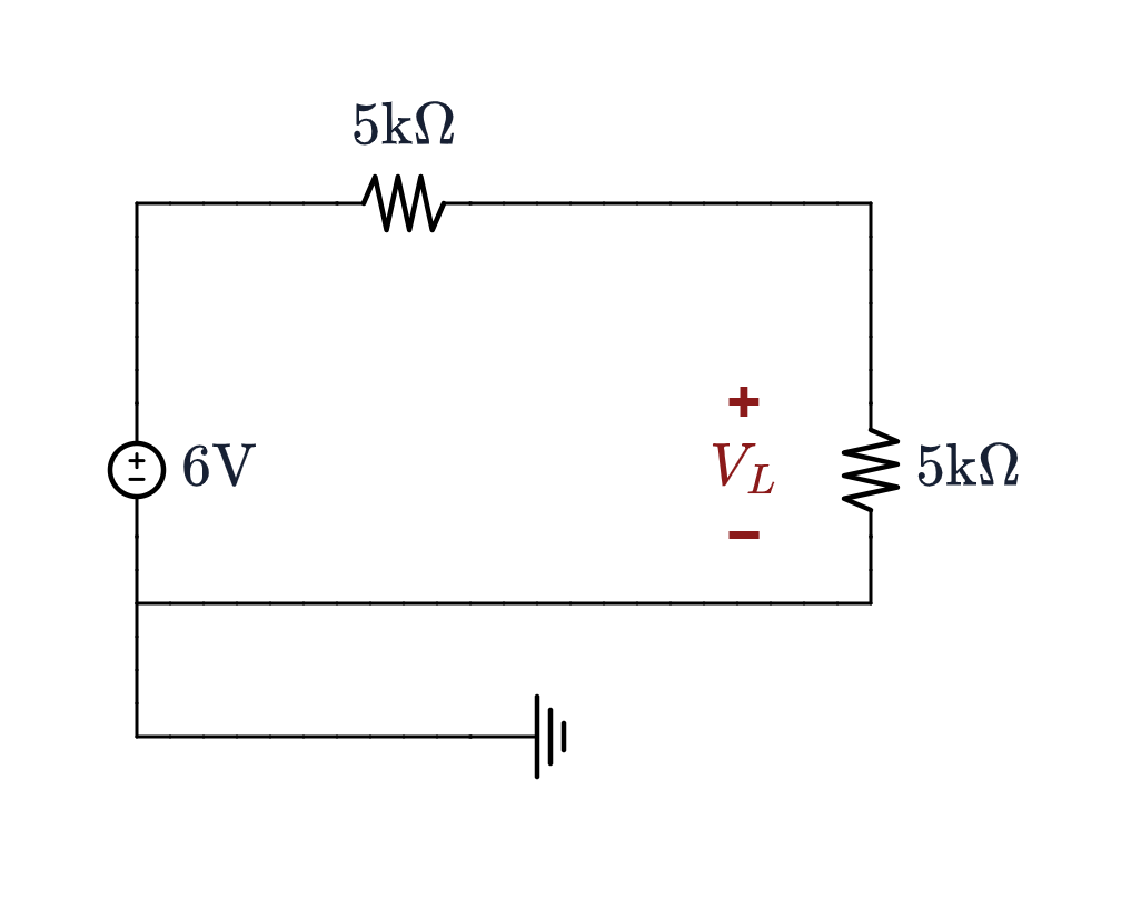
Worked Example 2 produced $V_{Th} = 6$ V behind $R_{Th} = 5\ \text{k}\Omega$. Which load draws the most power, and how much?
$$\begin{aligned} R_L &= R_{Th} = \mathbf{5\ \text{k}\Omega} \\ P_{max} &= \frac{6^2}{4(5\text{k})} = \frac{36}{20\text{k}} = \mathbf{1.8\ \text{mW}} \end{aligned}$$
| $R_L$ | $V_o$ | $P_L = V_o^2/R_L$ |
|---|---|---|
| $1\ \text{k}\Omega$ | $1$ V | $1.0$ mW |
| $5\ \text{k}\Omega$ | $3$ V | $\mathbf{1.8}$ mW |
| $10\ \text{k}\Omega$ | $4$ V | $1.6$ mW |
Same three loads as slide 18, now read as power. $V_o$ climbs all the way; $P_L$ turns over. And at the match the load sits at $3$ V — exactly half of $V_{Th}$, which is the quickest check that a circuit is matched.
The Caveat: Power Transferred Is Not Efficiency
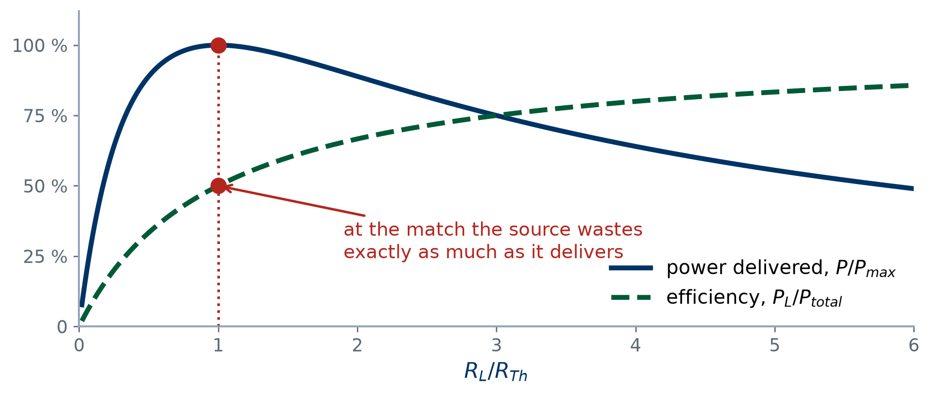
- At the match both resistances carry the same current and drop the same voltage, so $\eta = \mathbf{50\,\%}$: the source wastes as much as it delivers.
- Power systems are never matched — $R_{Th}$ is made as small as possible, so $\eta \to 100\,\%$. Signal circuits often are (antenna, sensor, audio out): there $R_{Th}$ is fixed by physics and the available power is tiny, so you take all you can get.
Part 2b: $R_{Th}$ When a Dependent Source Is Present
Every $R_{Th}$ so far came from case (a): zero the independent sources, then combine resistors. With a dependent source in the network that route is simply not available.
⚠️ Why you cannot “turn off” a dependent source
- An independent source is an input. Zeroing it is a legitimate question: what does the network do with one input removed?
- A dependent source is part of the network's description — it is how that transistor, that amplifier, that model behaves. Zeroing it does not analyse the network; it analyses a different network.
- And you could not hold it fixed either: its value follows a voltage or current elsewhere in the circuit, so it changes with whatever you connect to the terminals. You will watch that happen on the next slide but one.
Three Routes to $R_{Th}$, and When Each Works
| Route | What you do | Works when |
|---|---|---|
| (a) Reduce | Zero the independent sources; combine resistors looking into $a$–$b$. | Independent sources only. |
| (b) Test source | Zero the independent sources, leave the dependent ones alone, drive $a$–$b$ with $1$ V (or $1$ A) and find the current (or voltage) it takes: $R_{Th} = v_{test}/i_{test}$. | Always. |
| (c) $V_{oc}/I_{sc}$ | Find the open-circuit voltage and the short-circuit current of the network as it stands — nothing zeroed: $R_{Th} = V_{oc}/I_{sc}$. | Whenever $V_{oc} \neq 0$. |
- Dependent source present? Use (b) or (c). Route (c) is usually less work, because $V_{oc}$ is needed for $V_{Th}$ anyway — so the second calculation buys you both numbers.
- No independent sources at all? Then $V_{oc} = 0$, route (c) gives $0/0$, and (b) is the only one left. A network of resistors and dependent sources still has an $R_{Th}$; it just has no $V_{Th}$.
Worked Example 4: Step 1, the Open-Circuit Voltage
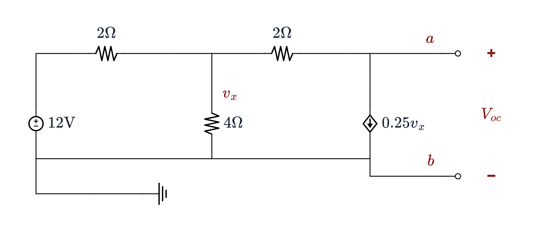
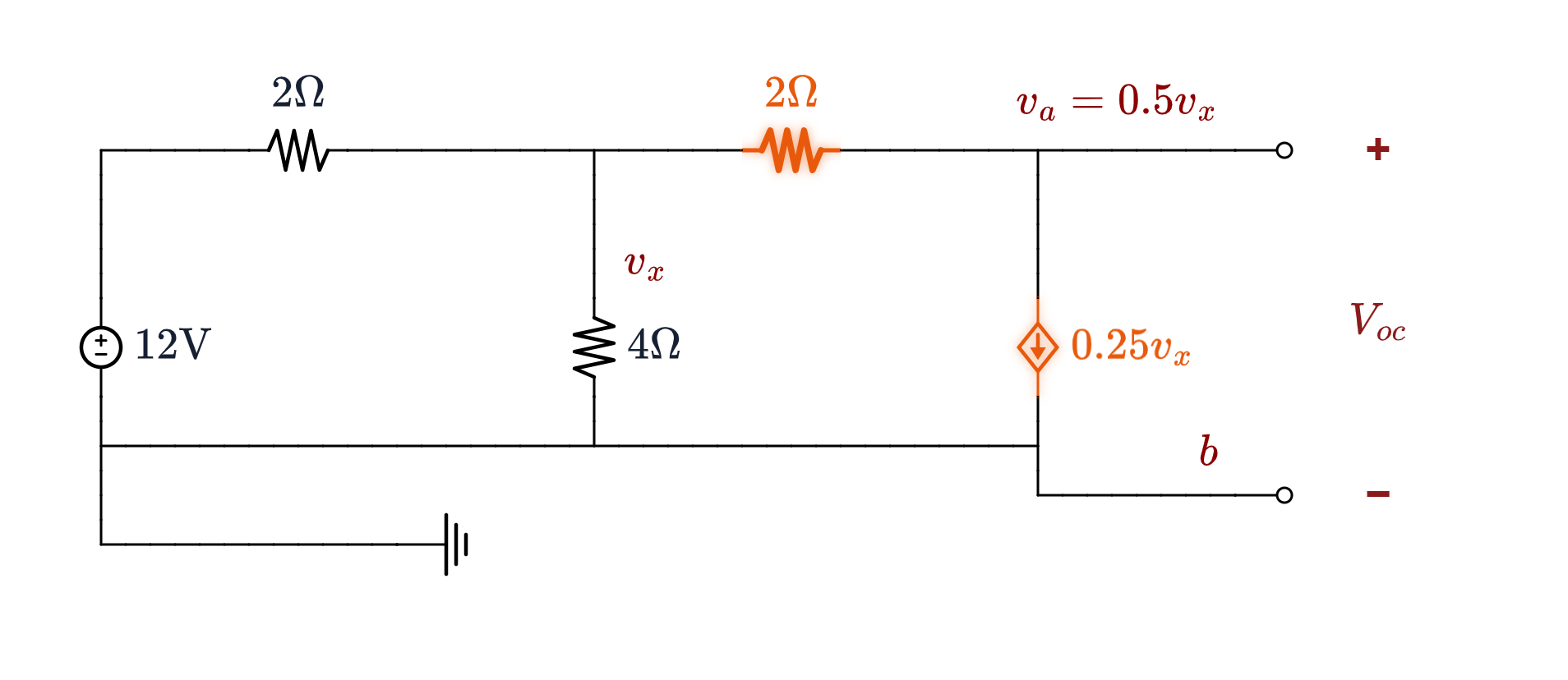
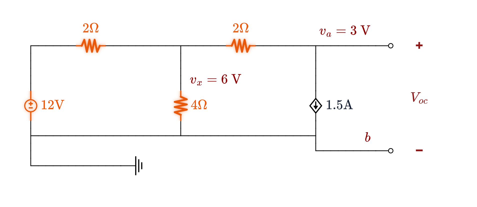
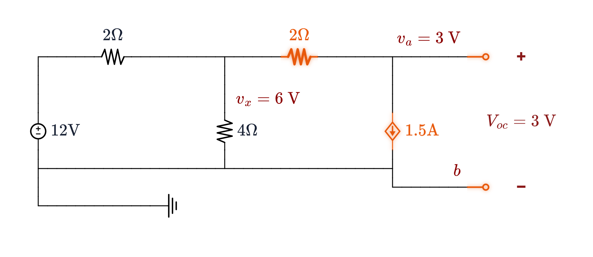
The diamond is a voltage-controlled current source: it pushes $0.25\,v_x$ amperes, where $v_x$ is the drop across the $4\ \Omega$. Find the Thévenin equivalent at $a$–$b$.
With $a$–$b$ open, everything the dependent source draws has to come through the $2\ \Omega$. KCL at $a$: $$\frac{v_a - v_x}{2} + 0.25\,v_x = 0 \;\Longrightarrow\; v_a = 0.5\,v_x$$
KCL at the $v_x$ node, with that substituted: $$\begin{aligned} \frac{v_x - 12}{2} + \frac{v_x}{4} + \frac{v_x - 0.5 v_x}{2} &= 0 \\ \Longrightarrow\quad 4v_x = 24 \quad&\Longrightarrow\quad v_x = 6\ \text{V} \end{aligned}$$
$$V_{Th} = V_{oc} = v_a = \mathbf{3\ \text{V}}$$
Step 2, Route (c): the Short-Circuit Current
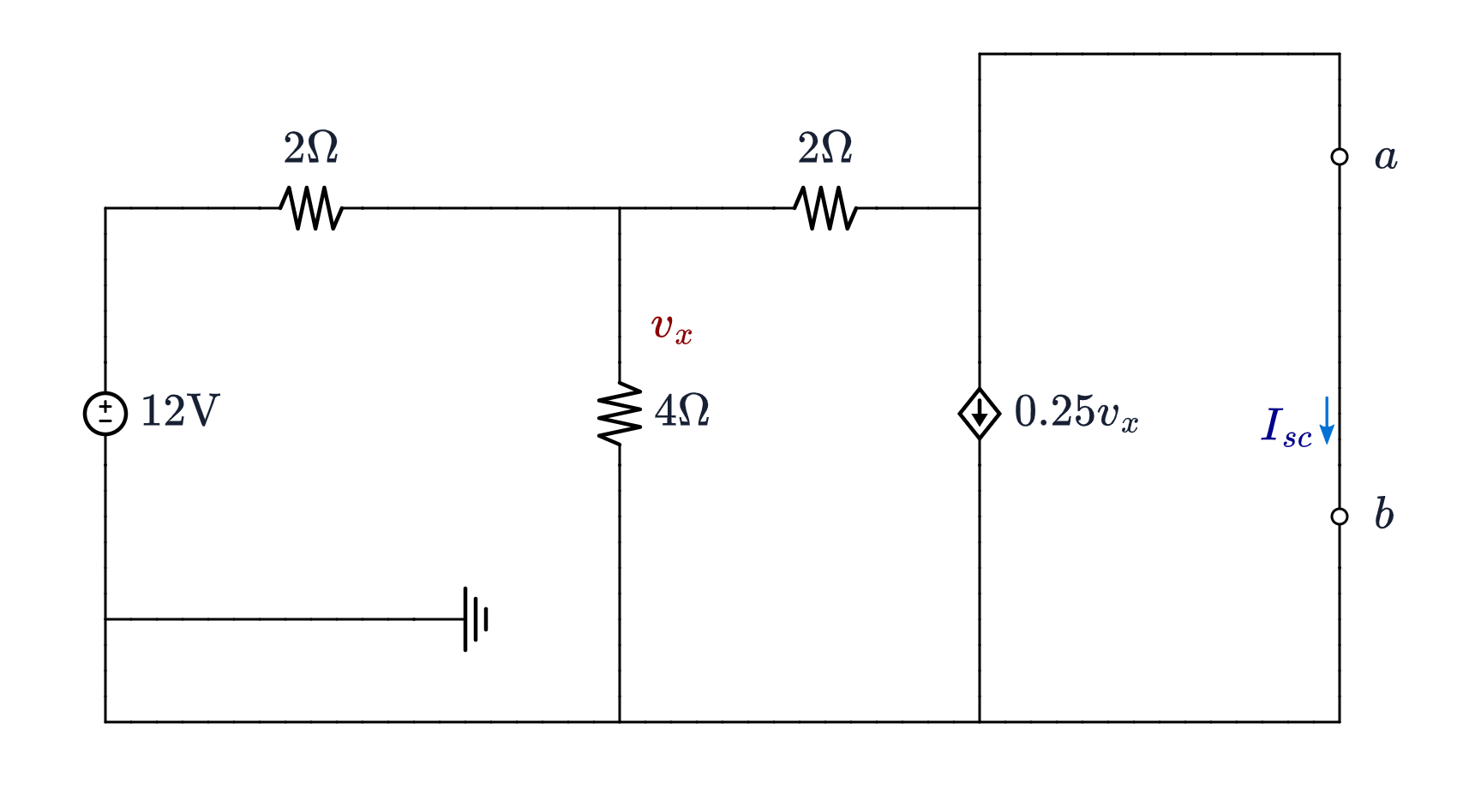
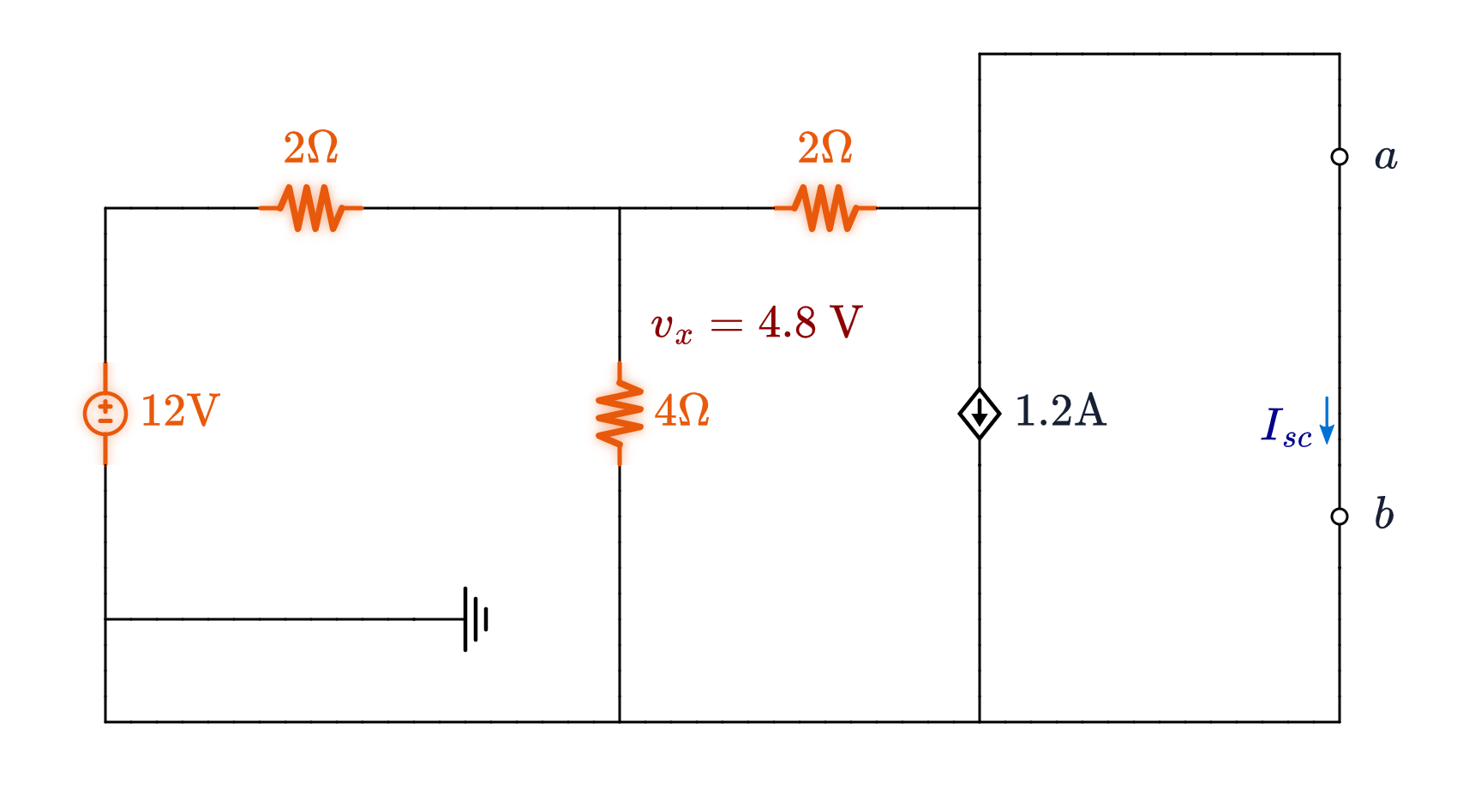
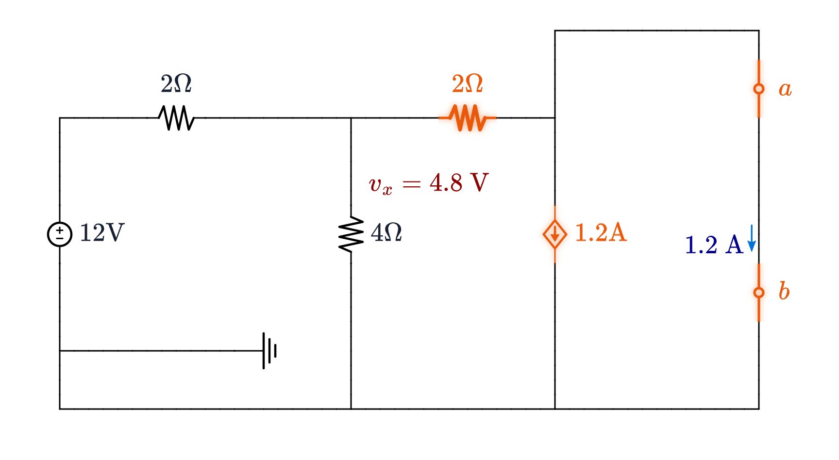
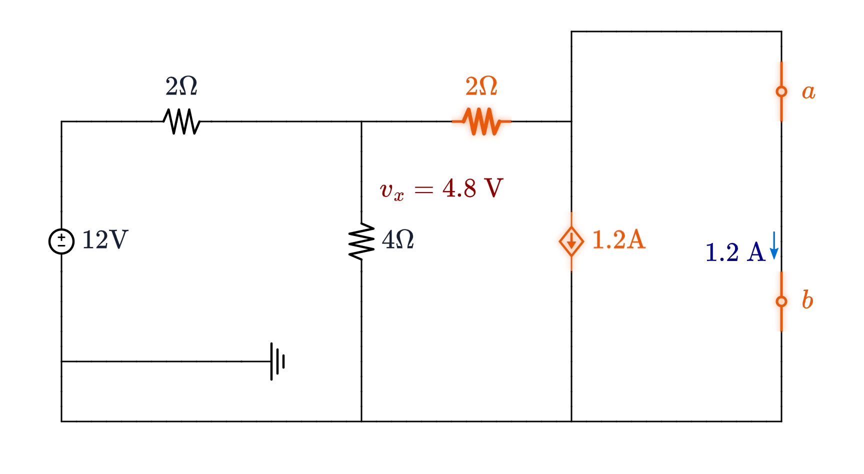
Short $a$–$b$, so $v_a = 0$. Solve for $v_x$, then find $I_{sc}$ through the short.
KCL at the $v_x$ node ($2\ \Omega$ now runs straight to ground): $$\begin{aligned} \frac{v_x - 12}{2} + \frac{v_x}{4} + \frac{v_x}{2} &= 0 \;\Longrightarrow\; 5v_x = 24 \;\Longrightarrow\; v_x = \mathbf{4.8\ \text{V}} \end{aligned}$$ $v_x$ moved — 6 V to 4.8 V (dependent source follows to $1.2$ A).
At node $a$, arriving current splits ($\frac{v_x}{2} = 0.25\,v_x + I_{sc}$): $$I_{sc} = \frac{v_x}{2} - 0.25\,v_x = 2.4 - 1.2 = \mathbf{1.2\ \text{A}}$$
$$R_{Th} = \frac{V_{oc}}{I_{sc}} = \frac{3}{1.2} = \mathbf{2.5\ \Omega}$$
Step 2, Route (b): the Test Source — Same Answer
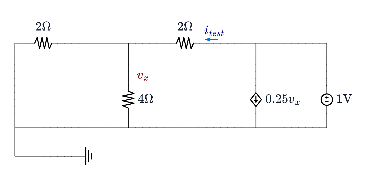
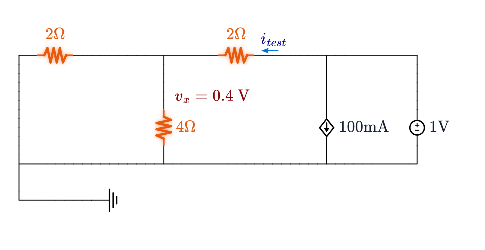
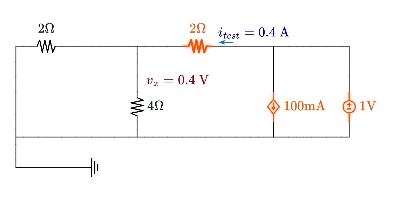
Zero independent source only; drive $a$–$b$ with $1$ V.
KCL at $v_x$: $$\frac{v_x}{2} + \frac{v_x}{4} + \frac{v_x - 1}{2} = 0 \;\Longrightarrow\; 5v_x = 2 \;\Longrightarrow\; v_x = \mathbf{0.4\ \text{V}}$$
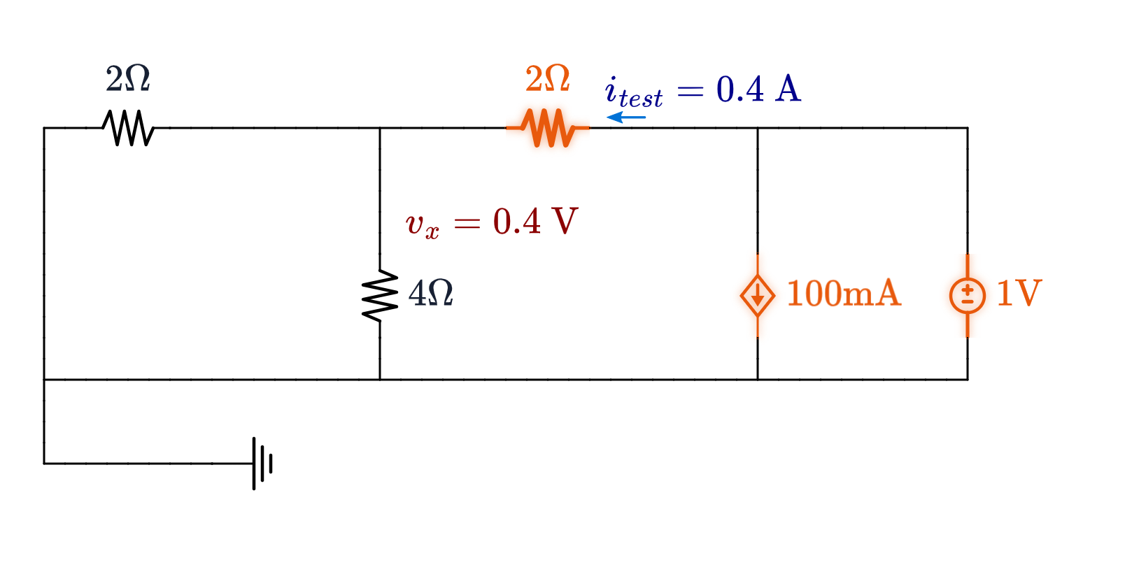
Current test source supplies ($2\ \Omega$ + dependent source): $$i_{test} = \frac{1 - v_x}{2} + 0.25\,v_x = 0.3 + 0.1 = \mathbf{0.4\ \text{A}}$$
$$R_{Th} = \frac{v_{test}}{i_{test}} = \frac{1}{0.4} = \mathbf{2.5\ \Omega} \quad\checkmark \quad\text{(same answer)}$$
Step 3: The Equivalent, and Its Best Load
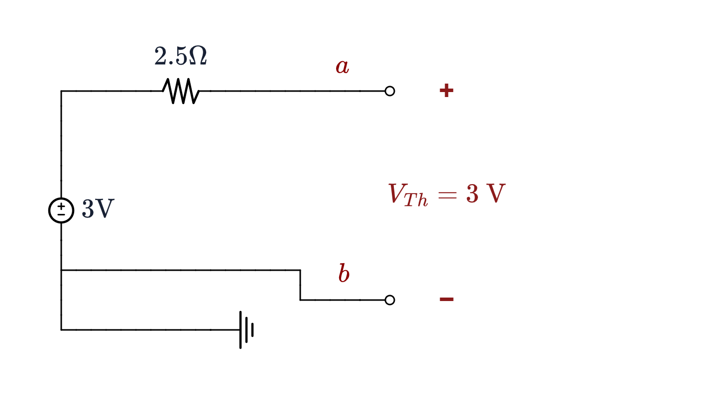
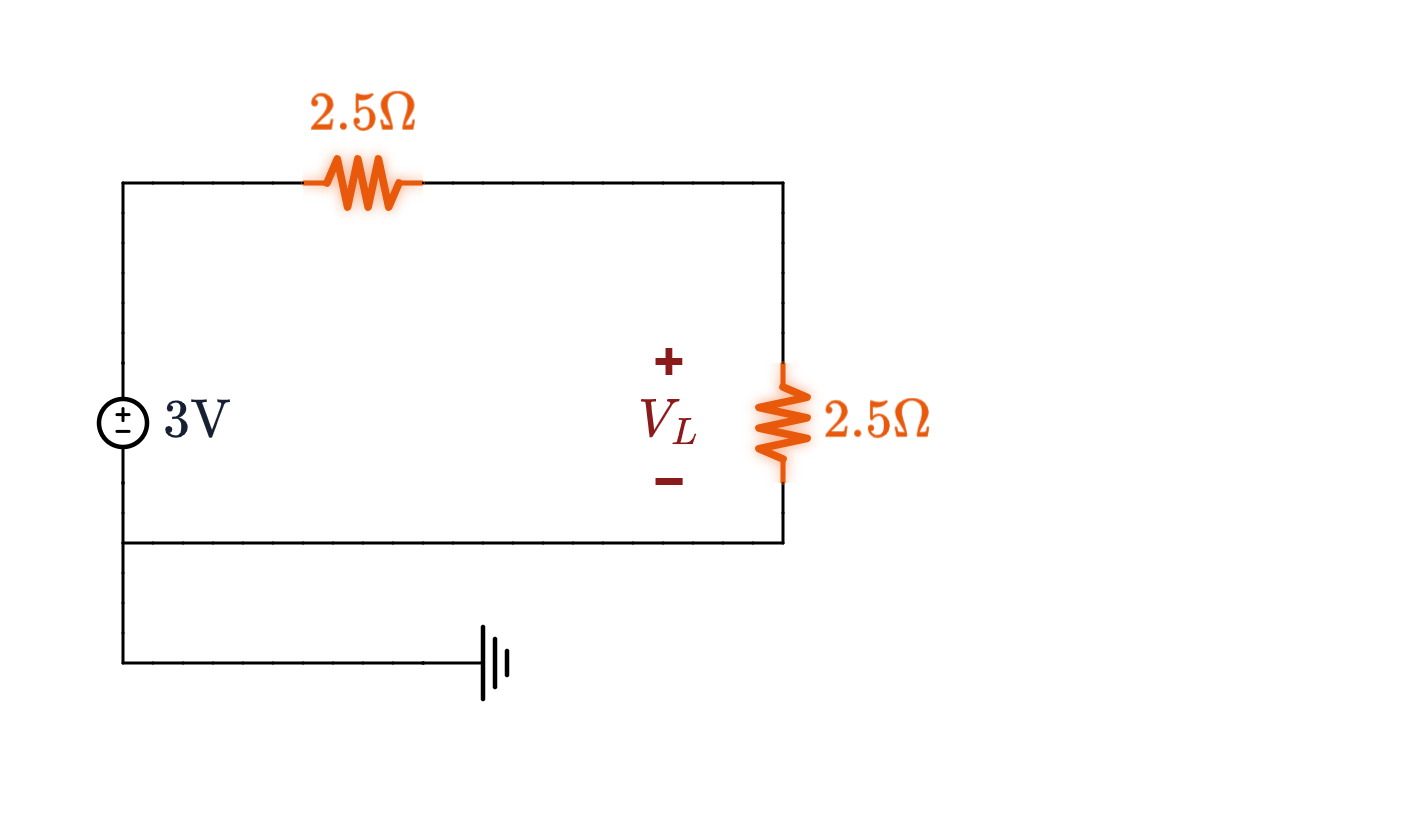
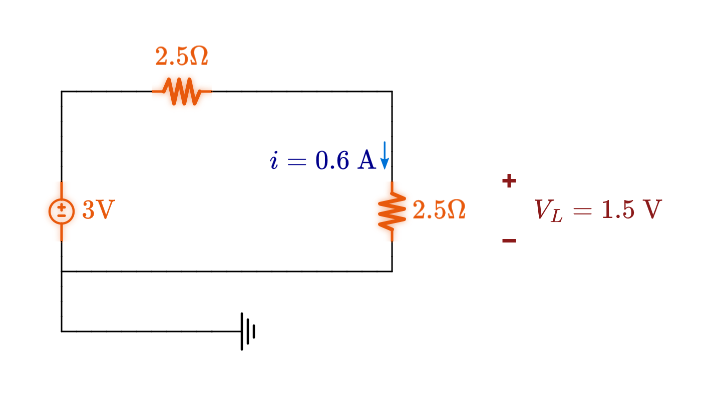
Four elements and a dependent source, replaced by two elements: $$V_{Th} = 3\ \text{V} \qquad R_{Th} = 2.5\ \Omega$$
Matched load and maximum power: $$R_L = R_{Th} = \mathbf{2.5\ \Omega} \qquad P_{max} = \frac{3^2}{4(2.5)} = \mathbf{0.9\ \text{W}}$$
Check: $i = 3/5 = 0.6$ A, $V_L = 1.5$ V (half of $V_{Th}$) — $P = (1.5)(0.6) = \mathbf{0.9\ \text{W}}$. ✓
Hang $2.5\ \Omega$ on the original network and it also reads $1.5$ V.
Traps
| Trap | What goes wrong |
|---|---|
| Zeroing the dependent source | Gives $R_{Th} = (2\,\|\,4) + 2 = 3.33\ \Omega$ here instead of $2.5\ \Omega$ — a plausible-looking number for a different circuit. |
| Carrying $v_x$ over from one step to the next | $v_x$ is $6$ V open and $4.8$ V shorted. Reusing $6$ V gives $I_{sc} = 1.5$ A and $R_{Th} = 2\ \Omega$. |
| $R_L = R_{Th}$ read as “$R_L$ equals some resistor in the circuit” | $R_{Th}$ is the resistance looking in from the load's terminals. Here nothing in the network is $2.5\ \Omega$. |
| $P_{max} = V_{Th}^2/R_{Th}$ | Four times too big. Half of $V_{Th}$ is across the load at the match, so the $4$ is not optional. |
| Matching when efficiency is what matters | Correct arithmetic, wrong question — see slide 24. |
Summary, and What Comes Next
📝 Deck 07, both parts
- Source transformation: $v_S = R\,i_S$, either direction, terminals unchanged.
- Thévenin / Norton: any linear network at two terminals is one source and one resistor, with $I_N = V_{Th}/R_{Th}$ and $R_N = R_{Th}$.
- $R_{Th}$, three routes: reduce (independent only), test source (always), $V_{oc}/I_{sc}$ (whenever $V_{oc} \neq 0$).
- Maximum power: $R_L = R_{Th}$, $P_{max} = V_{Th}^2/4R_{Th}$, at $50\,\%$ efficiency and with a broad peak.
- Assignment 2 is issued today, due Wednesday 30 September. It uses superposition, both equivalents, source transformation, and maximum power transfer — including a network with a dependent source, which is Worked Example 4's shape.
- Thursday: energy storage begins. Capacitors — the $v$–$i$ relationship, stored energy, and series/parallel combinations (Irwin Ch. 6, Sec. 6.1–6.2). Every circuit so far has been resistive and memoryless; that ends.